
Ein Ansatz zur formalen Verifikation von neuronalen Netzen im Detail
In dem ersten Teil dieses Blogs haben wir die folgende Aufgabe ausführlich beschrieben: „Wie lassen sich menschlich verständliche Sicherheitskriterien für neuronale Netze in ein korrektes und vollständiges mathematisches Problem übersetzen, das beweisbar ist?“. Dafür werden wir weiterhin ein neuronales Netz zur Erkennung von Verkehrszeichen referenzieren, welches mit unterschiedlichen Beleuchtungssituationen zurechtkommen muss.
Welches Verhalten genau abgesichert wird
Die verschiedenen Beleuchtungssituationen werden in unserem Beispiel durch photometrische Transformationen modelliert. Somit wird die Robustheit des neuronalen Netzes gegenüber ebendiesen photometrischen Transformationen geprüft. Solche Transformationen sind z.B. die Änderung von Helligkeit oder Kontrast.
In diesem Beispiel beschränken wir uns auf die Verringerung des Kontrastes um bis zu 50% des ursprünglichen Wertes. Betrachten wir ein potenzielles Eingangsbild für ein neuronales Netz x mit den Farbkanälen c_{in}, der Höhe h_{in} und der Breite w_{in}, so wird die folgende Formel verwendet:
\,\,\,\,\,\,\,\,{x}'_{c,h,w}=\alpha\cdot x_{c,h,w}\,\,\,\,\alpha \in [0.5,1],
wobei der Faktor \alpha die Verringerung des Kontrastes beschreibt.
Für mehr Hintergrundinformationen zu dem Thema „photometrische Transformationen“ bietet die Dokumentation von OpenCV eine gute Übersicht: https://docs.opencv.org/3.4/d3/dc1/tutorial_basic_linear_transform.html
Damit haben wir den Punkt erreicht, an dem die Übersetzung unserer Aufgabe in die Form einer Mixed-integer linear programming (MILP) Kodierung beginnt.
Die betrachtete Transformation wird auf jeden Pixel in jedem Farbkanal des Originalbildes gleich angewandt. Es ergeben sich somit die ersten c_{in}\cdot h_{in}\cdot w_{in} Constraints:
\; \; \; \;constr\left ( c,h,w \right ):\, {x}'_{c,h,w}=\alpha \cdot x_{c,h,w}\\
\; \;\; \; c=0, …, c_{in}-1\; \:\; \; h=0, …, h_{in}-1\; \; \; \;w=0, …,w_{in}-1
Und die erste Boundary für eine Variable:
\; \; \; \;boundary(1):\; 0.5\leq \alpha \leq 1
Die Variablen stehen dabei für:
c_{in},\,h_{in},\,w_{in} Anzahl der Farbkanäle, Höhe und Breite des Bildes
x Originalbild
{x}'\, transformiertes Bild
Wenn das neuronale Netz z.B. RGB-Bilder mit einer Auflösung von 640\cdot 480 Pixel verarbeiten soll, dann ergeben sich somit bereits 921601 (Un-)Gleichungen!
Die Kodierung des neuronalen Netzes als MILP
An dieser Stelle möchten wir in einer (verhältnismäßig) knappen Form die MILP-Kodierung der gängigsten Layer neuronaler Netze vorstellen. Die Layer selbst werden konzeptionell nicht erklärt und als Hintergrundwissen vorausgesetzt. Eine gute Referenz für die Notationen, die in diesem Blog verwendet werden, bietet die Dokumentation von pytorch: https://pytorch.org/docs/stable/nn.html
Fully–Connected Layer
Da Fully-Connected Layer lediglich gewichtete Summen darstellen, können diese ohne Weiteres als lineare Gleichungen dargestellt werden. Dabei wird für jedes (Ausgangs-)Neuron in dem Layer ein Constraint benötigt:
constr(n):\, {x}'_{n}=b_{n}+\sum_{i=0}^{n_{in}-1}a_{n,i}\cdot x_{i}\: \:\: \: \:\: n=0, …, n_{out}-1
Die Variablen stehen dabei für:
n_{in} Anzahl der Eingangswerte / Neuronen im vorherigen Layer
n_{out} Anzahl der Ausgangswerte / Neuronen im aktuellen Layer
x Vektor mit n_{in} Eingangswerten
{x}'\, Vektor mit n_{out} Ausgangswerten
b_{n} Bias der gewichteten Summe für das n-te Neuron des aktuellen Layers
\alpha_{n} Vektor mit Faktoren der gewichteten Summe für das n-te Neuron des aktuellen Layers
Convolutional Layer
Konzeptionell sind Convolutional Layer den Fully-Connected Layern sehr ähnlich, da beide gewichtete Summen darstellen. Um die Darstellung übersichtlich zu halten, werden Padding, Stride und Dilation in den Formeln und Constraints in dieser Erklärung vernachlässigt:
constr(c,h,w):\; {x}'_{c,h,w}=b_{c}+\sum_{i=0}^{c_{k}-1}\sum_{j=0}^{h_{k}-1}\sum_{l=0}^{w_{k}-1}\alpha_{i,j,l}\cdot x_{c+i,h+j,w+l}\\
c=0, …,c_{out}-1\;\; \: h=0, …,h_{out}-1\; \;\;\; \; w=0, …,w_{out}-1
Die Variablen stehen dabei für:
c_{out}\,, h_{out}\,, w_{out} Anzahl der Channel, Höhe und Bereite des Ausgangstensors x'\, (wie diese genau
in Abhängigkeit von der Größe des Kernels, Stride, Padding und Dilation berechnet
werden können, kann ebenfalls der pytorch Dokumentation entnommen werden:
https://pytorch.org/docs/stable/generated/torch.nn.Conv2d.html)
c_{in} Anzahl der Channel des Eingangstensors x
\alpha 3-dimensionaler Tensor mit Gewichtsfaktoren (Kernel)
b_{c} Bias der gewichteten Summe für den Channel mit Index c_{k}\,, h_{k}\,, w_{k} Anzahl
der Channel (gleich der Anzahl der Channel des Eingangstensors x ),
Höhe und Breite des Kernels \alpha
x 3-dimensionaler Eingangstensor (z.B. Bild)
{x}'\, 3-dimensionaler Ausgangstensor
ReLU-Aktivierung
ReLU-Aktivierungen sind wie folgt definiert:
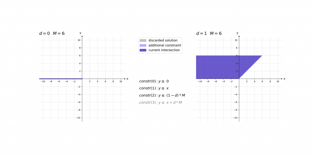
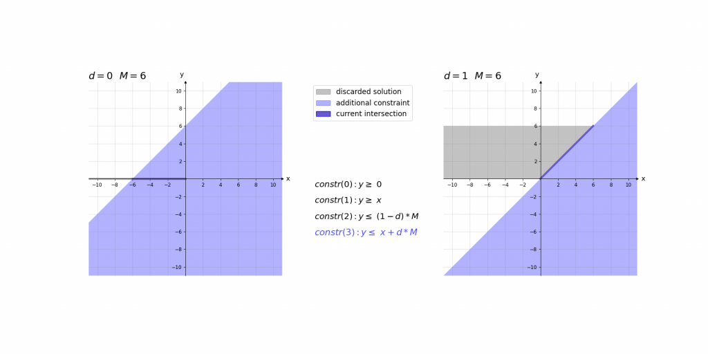
ReLU\left ( x \right )=y=max(0,x)=\left\{\begin{matrix} x & if\, x> 0\\ 0 & if\, x\leq 0 \end{matrix}\right.Da ReLU-Aktivierungen nur teilweise linear sind, werden für die MILP-Kodierung hier Hilfsmittel benötigt. Diese benötigten Hilfsmittel sind zwei Variablen: Eine binäre „Entscheidungsvariable“ d ∈ {0,1} und eine Hilfsvariable M, die nur einen ausreichend großen Wert haben muss. „Ausreichend groß“ heißt in diesem Fall, dass sie größer als die möglichen Eingangswerte x sein muss.
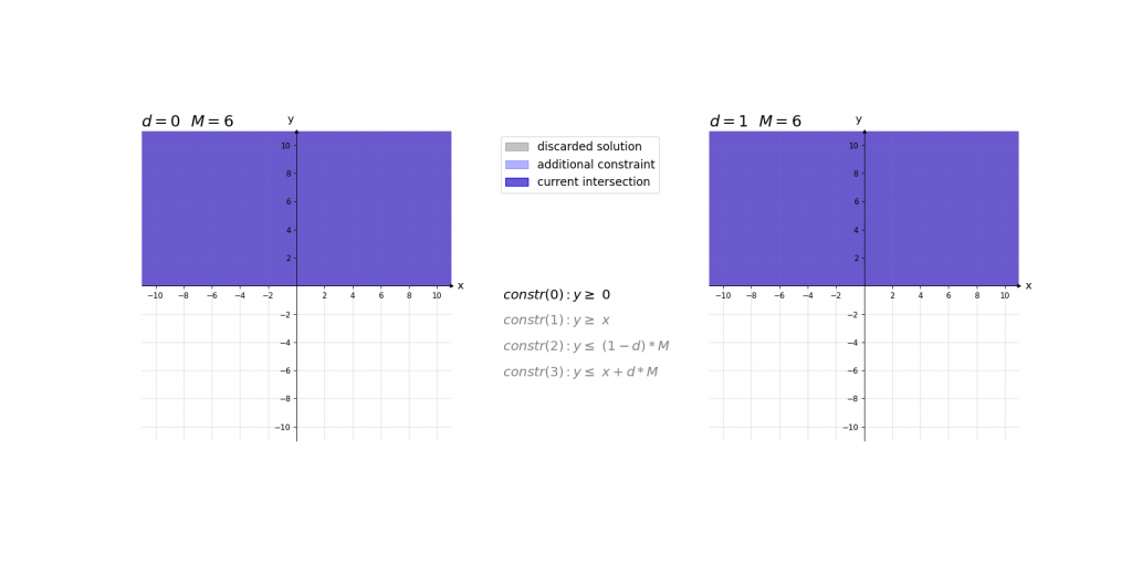
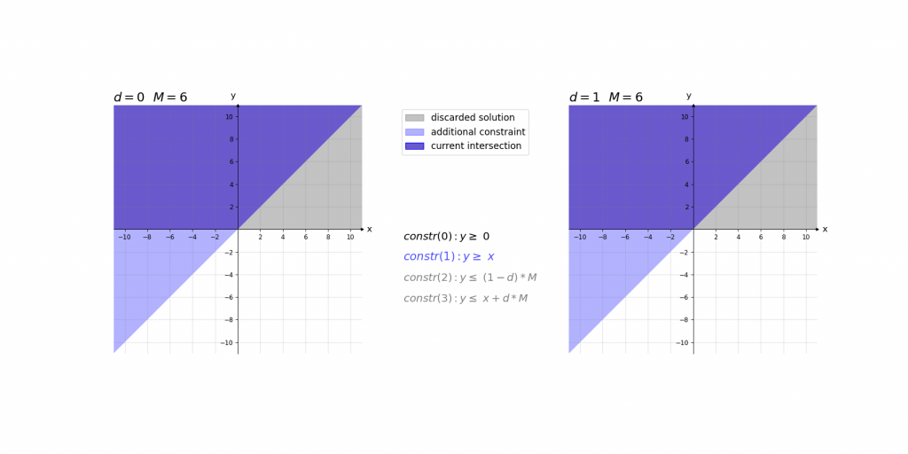
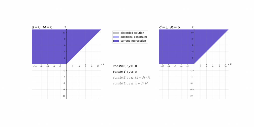
Für die Erklärung der Kodierung betrachten wir zunächst die fertigen Constraints der ReLU-Aktivierung für einen einzelnen Wert und erklären diese daraufhin:
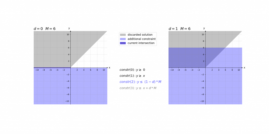
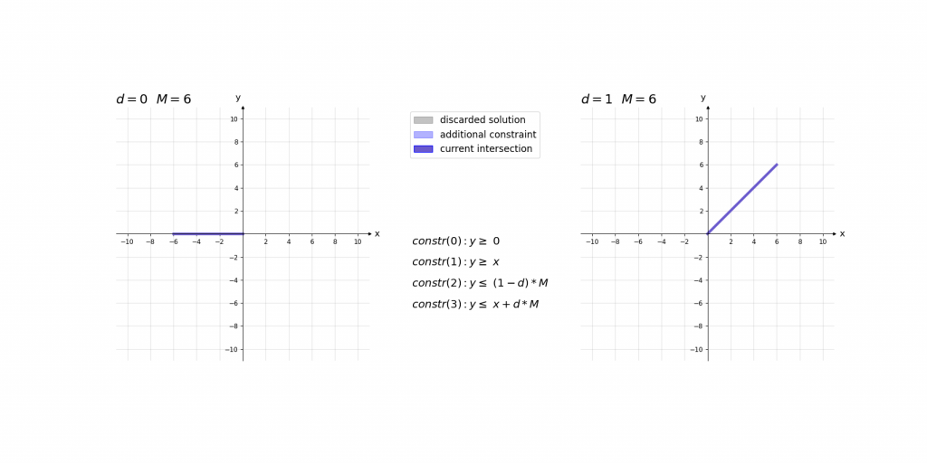
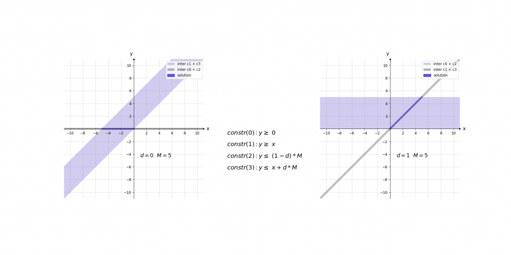
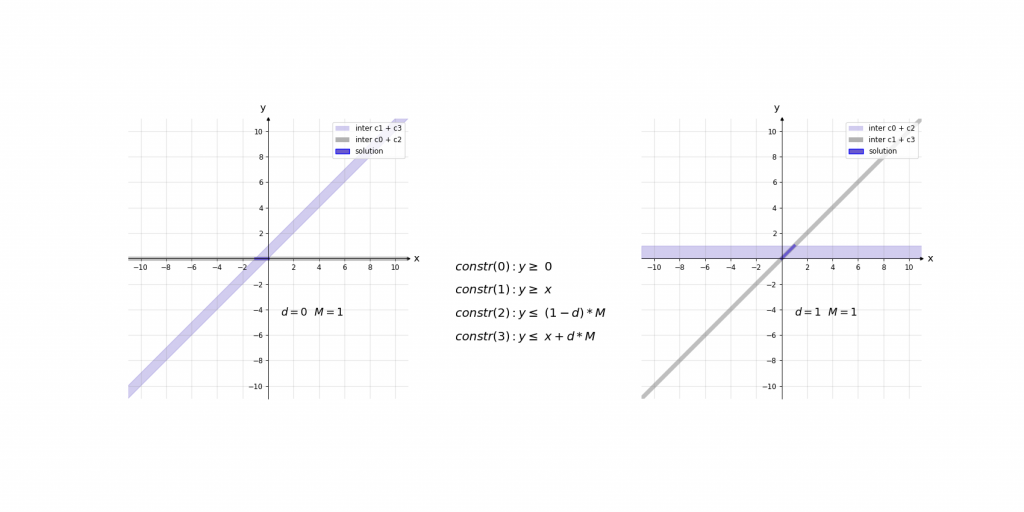
\,\,\,\,constr(0):\,\,\,\,\,\,\,\,y\geq 0\\ \,\,\,\,constr(1):\,\,\,\,\,\,\,\,y\geq x\\ \,\,\,\,constr(2):\,\,\,\,\,\,\,\,y\leq d\cdot M\\ \,\,\,\,constr(3):\,\,\,\,\,\,\,\,y\leq x+(1-d)\cdot M\\ \,\,\,\,boundary(0):d \in \left \{ 0,1 \right \}\\ \,\,\,\,boundary(1): M=1000Bei der Erklärung kann es helfen das Ergebnis der ReLU-Aktivierung einfach als das Maximum y von zwei Werten (0 und x) im Sinn zu haben. Die ersten beiden Constraints constr(0) und constr(1) sagen lediglich aus, dass dieses Maximum y größer gleich der beiden Eingangswerte 0 und x ist. Dies würde jedoch noch unendlich viele Werte y zulassen. Da d entweder 0 oder 1 ist ergibt sich durch constr(2) und constr(3), dass das Maximum y entweder kleiner gleich 0 oder x ist.
Die Contraints haben dabei die Form, dass abhängig von x nur eine Belegung von d für ein zulässiges Gleichungssystem sorgt. Dieses hat dann entweder die Lösung x\leq y\leq x oder 0\leq y\leq 0 . Somit haben diese 4 Gleichungen immer nur eine zulässige Variablenbelegung , die nur genau eine Lösung für y zulässt.
Beispiel:
M = 1000
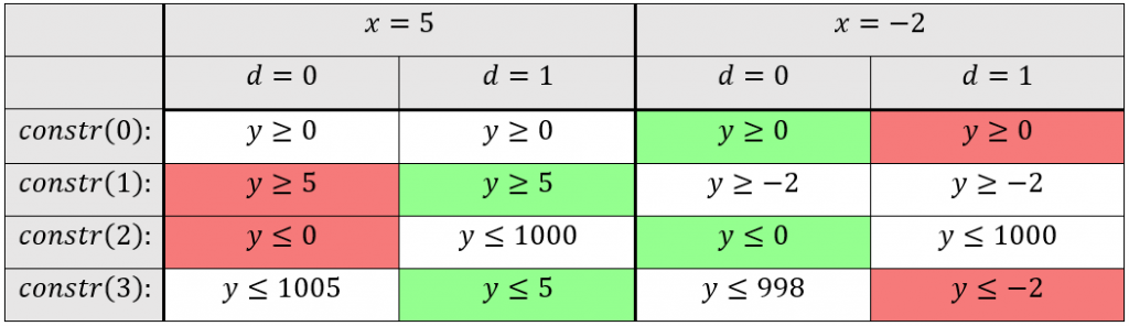
*rot markierte Felder stellen einen Widerspruch dar, während grün markierte Felder zeigen, welche Constraints den Lösungswert für y bestimmen.
Visualisierung:
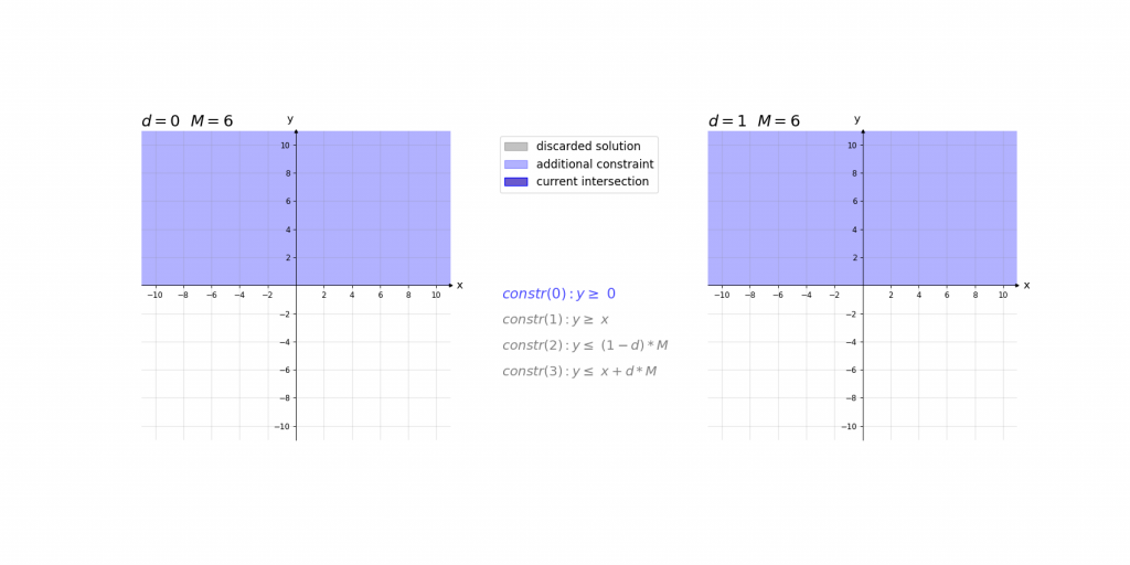
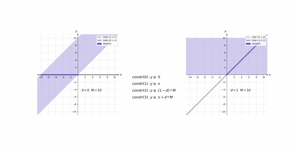
Visualisierung des Einflusses von M:
Max-Pooling
Die Kodierung von Max-Pooling-Operationen kann im Groben als eine Kombination aus Convolutional Layer und ReLU verstanden werden. Jedoch gibt es nicht wie bei der ReLU nur 2 Kandidaten für das Maximum, sondern entsprechend der Größe des Max-Pooling-Kernels mehr. Jeder Kandidat bekommt für das Maximum 2 Constraints und eine binäre Variable. Zusätzlich wird je Berechnung eines Maximums ein weiteres Constraint benötigt, um genau ein Maximum zu bestimmen. Da dies von der Indizierung recht komplex wäre, obwohl Stride, Padding und Dilation bereits in der Erklärung vernachlässigt werden, lohnt es sich für das Verständnis nur eine einzelne Berechnung des Maximums anzusehen:
\;\;\;\;constr(1):\; \;\;\;\;\;\;\;\;\;\;1=\sum_{i=0}^{h_{k}}\sum_{j=0}^{w_{k}}d_{i,j}\\
\;\;\;\;constr(m,n,1):\;\;\;y\geq x_{m,n}\\
\;\;\;\;constr(m,n,2):\;\;\;y\leq x_{m,n}+(1-d_{m,n})\cdot M\\
\;\;\;\;boundary(0):\;\;\;\;\;\;\; M=1000\\
\;\;\;\;boundary(m,n):\;\;\; d_{m,n}\in \left \{ 0,1 \right \}\\
\;\;\;\;m= 0, …,h_{k}-1\: \: \: \:n=0, …,w_{k}-1
Die Variablen stehen dabei für:
h_{k}\,, w_{k} Höhe und Breite des Max-Pooling-Kernels
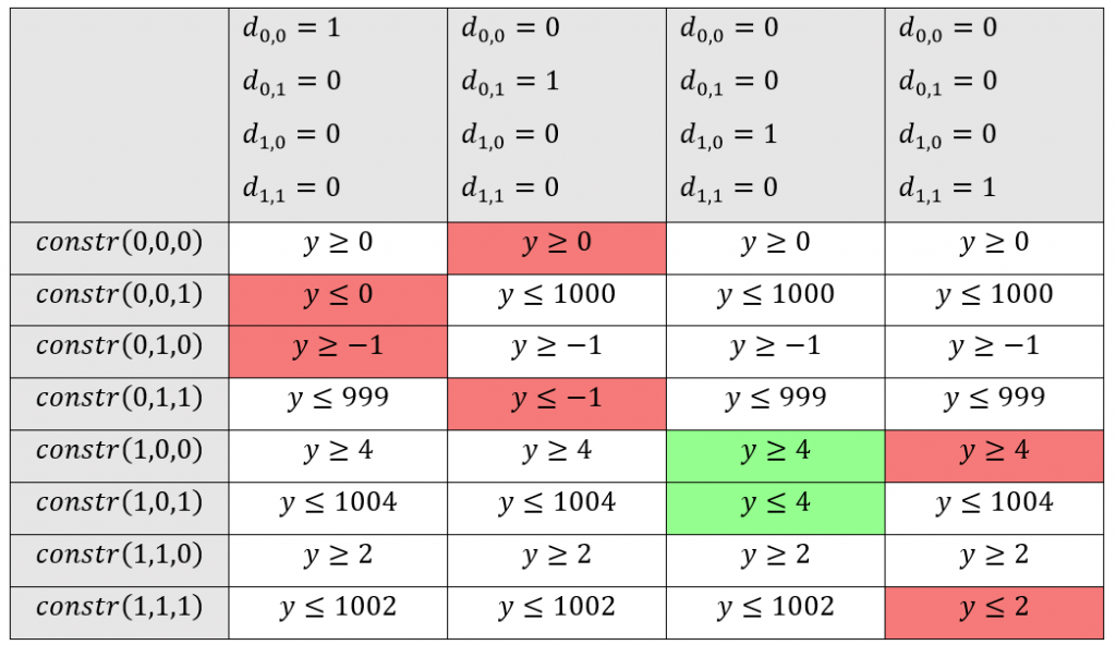
Beispiel:
Wir gehen direkt davon aus, dass constr(1) erfüllt ist und somit die Summe aller Binärvariablen d_{i,j} gleich 1 ist. In diesem Beispiel wird ein Max-Pooling-Kernel mit der Größe 2 x 2 verwendet. Die Matrix der Kandidaten für das Maximum ist dabei:
Sicherheitskriterien für Klassifikationsprobleme
Der dritte Teil der Kodierung, neben den Transformationen und dem neuronalen Netz, ist das jeweilige Sicherheitskriterium. Dieses Sicherheitskriterium beschreibt die Eigenschaften für sicheres Verhalten und ermöglicht somit ebenfalls das ableiten eines Beispiels, welches die Robustheit widerlegt. Das Sicherheitskriterium wird also auch als Menge von Constraints in Abhängigkeit der Aufgabe des neuronalen Netzes (Klassifikation, Regression, Objekterkennung, …) abgebildet. Sicherheitskriterien im Allgemeinen basieren auf dem Prinzip, dass abhängig von einem bekannten Eingangswert x und definierten Transformationen kein Eingangswert {x}'\,abgeleitet werden kann, der ungewollte Verhalten mit sich bringt.
Im Falle der Klassifikation ist dieses Kriterium, dass sich das Klassifikationsergebnis trotz Veränderungen des Eingangsbildes durch die definierten (photometrischen) Transformationen nicht ändert. Dafür gehen wir davon aus, dass die möglichen Klassen im Output-Layer one-hot-encoded sind. Das Neuron mit der höchsten Aktivierung, welches die prädizierte Klasse bestimmt, nennen wir im folgenden Gewinner-Neuron.
Da das Verfahren auf dem Konzept des Widerspruchbeweises aufbaut, wird nach Gegenbeispielen für Robustheit gesucht. Für die Klassifikation ergibt sich daher, dass solch ein Gegenbeispiel bei einem anderen als dem ursprünglichen Gewinnerneuron den höchsten Aktivierungswert hat.
Dieses Kriterium kann mit den folgenden Constraints ausgedrückt werden:
\; \; \;\;constr(i):\;\;\;\;\;\;\;\;\;\;\;\;\;\;\;\;\;\;\; x_{i}+(1-d_{i})\cdot M\geq x_{idx_{o\verb|_|p}}\\ \; \; \;\; constr(n_{classes}+1):\;\;\;\;\; 1\geq \sum d_{i}\\ \; \; \;\;boundary(i):\;\;\;\;\;\;\;\;\;\;\;\;\;\;\; d_{i}\in \left \{ 0,1 \right \}\\ \; \; \;\;boundary(n_{classes}+1):M=1000\\ \; \; \;\;i=1, …,n_{classes}\wedge i\neq idx_{o\verb|_|p}Die Variablen stehen dabei für:
d_{i} binäre Variable
M ausreichend großer Wert (zur Erfüllung von constr(i))
n_{classes} Anzahl der möglichen Klassen / Output-Neuronen
x Vektor der Länge n_{classes} mit den Aktivierungswerten des Output-Layers
idx_{o\verb|_|p} Index des ursprünglichen Gewinner-Neurons
Die Constraints constr(i) sind dann erfüllt, wenn entweder die Aktivierung des jeweiligen output-Neurons höher ist als die Aktivierung des ursprünglichen Gewinner-Neurons oder ein Wert aufsummiert wird. Damit dieser Summand (1-d_{i} )\cdot M für die Erfüllung des jeweiligen Constraints constr(i) sorgt, muss die zugehörige binär Variable d_{i} den Wert 0 haben.
Das Constraint constr(n_{classes}+1) fordert jedoch, dass mindestens eine binäre Variable d_{i} gleich 1 ist und somit der Aktivierungswert das mindestens eines anderen Output-Neurons höher ist, als die des ursprüngliche Gewinner-Neurons.
Wenn eine zulässige Lösung existiert, liefert der MILP-Solver das entsprechende Gegenbeispiel und widerlegt somit die Robustheit der KI. Wenn jedoch kein Gegenbeispiel gefunden werden kann, beweist dies die Robustheit der KI.
Abschließende Worte
In diesem Teil des Blogs haben wir einen Einblick in unsere Arbeiten zu dem Thema der formalen Verifikation von KI-basierten (Fahr-)Funktionen geboten. Die hier präsentierten Kodierungen sind dabei nur ein Teil der Transformationen, Operationen und Sicherheitskriterien, mit denen wir uns im Rahmen dieses Ansatzes beschäftigen.
Wenn ihr mehr wissen möchtet, dann freuen wir uns von euch zu hören!
English Version
Part 2 of 2: an approach for the formal verification of neural networks in detail
In the first part of this blog, we described the following task: „How can we translate human-understandable safety criteria for neural networks into a correct and complete mathematical problem which can be proven?“. As an example, we will continue to look at a neural network for traffic sign recognition, which must be able to cope with different lighting situations.
What behavior is verified exactly?
In our example, the different lighting conditions are modeled by photometric transformations. Thus, the robustness of the neural network against those photometric transformations is checked. Such transformations are for example the change of brightness or contrast.
For this article, we look at a reduction of the contrast by up to 50% of the original value. If we consider a potential input image for a neural network x with color channels c_{in}, height h_{in} and width w_{in}, we can describe the contrast reduction formally as follows:
\,\,\,\,\,\,\,\,{x}'_{c,h,w}=\alpha\cdot x_{c,h,w}\,\,\,\,\alpha \in [0.5,1],
where \alpha is the factor to describe the reduction of the contrast.
For more background information on the topic „photometric transformations“, the documentation of OpenCV offers a good overview: https://docs.opencv.org/3.4/d3/dc1/tutorial_basic_linear_transform.html
This brings us to the point where the translation into the form of a Mixed-integer linear programming (MILP) encoding begins.
In our example of contrast reduction, the considered transformation is applied identically to every pixel in every color channel of the original image, resulting in the first c_{in}\cdot h_{in}\cdot w_{in} constraints:
\; \; \; \;constr\left ( c,h,w \right ):\, {x}'_{c,h,w}=\alpha \cdot x_{c,h,w}\\
\; \;\; \; c=0,\ …, c_{in}-1\;\; \; \: h=0, …, h_{in}-1\;\; \; \: w=0, …,w_{in}-1
And a single boundary for a variable:
\; \; \; \;boundary(1):\; 0.5\leq \alpha \leq 1
With the variables:
c_{in},\, h_{in},\, w_{in} number of color channels, heights and width of the image
x original image
{x}'\, transformed image
For example, if the neural network processes RGB images with a resolution of 640\cdot 480 pixels, then there are already 921601 (in-)equations!
The Encoding of Neural Networks as a MILP
At this point we present the MILP encoding of the most common layers of neural networks in a (relatively) brief form. The layers themselves are not explained conceptually and are assumed to be background knowledge. A good reference for the notations used in this blog is the pytorch documentation: https://pytorch.org/docs/stable/nn.html
Fully–Connected Layer
Because fully-connected layers only represent weighted sums, they can easily be represented as linear equations. For each (output-)neuron in the layer one constraint is required:
constr(n):\, {x}'_{n}=b_{n}+\sum_{i=0}^{n_{in}-1}\alpha_{n,i}\cdot x_{i}\: \:\: \: n=0, …, n_{out}-1
With the variables:
n_{in} number of input values / neurons in the previous layer
n_{out} number of output values / neurons in the current layer
x vector with n_{in} input values
{x}'\, vector with n_{out} output values
b_{n} bias of the weighted sum for the n-th neuron of the current layer
\alpha_{n} vector of weighted sum factors for the n-th neuron of the current layer
Convolutional Layer
Conceptually convolutional layers are very similar to fully-connected layers since both represent weighted sums. To keep this overview clear, padding, stride and dilation are neglected in the formulas and constraints in this explanation:
constr(c,h,w):\; {x}'_{c,h,w}=b_{c}+\sum_{i=0}^{c_{k}-1}\sum_{j=0}^{h_{k}-1}\sum_{l=0}^{w_{k}-1}\alpha_{i,j,l}\cdot x_{c+i,h+j,w+l}\\ c=0, …,c_{out}-1\;\;\;\; \: h=0, …,h_{out}-1\;\;\; \; \; w=0, …,w_{out}-1With the variables:
c_{out},\, h_{out},\, w_{out} number of channels, height and width of the output tensor {x}'\, (how those are
calculated in dependence of kernel size, stride, padding and dilation can also be
checked in the pytorch documentation:
https://pytorch.org/docs/stable/generated/torch.nn.Conv2d.html
c_{in} number of channels of the input tensor x
\alpha 3-dimensional tensor with weight factors (kernel)
b_{c} bias of the weighted sum for the channel with index c
c_{k},\, h_{k},\, w_{k} number of channels (equal to the number of channels of the input tensor x ),
height and width of the kernel \alpha
x 3-dimensional input tensor (e.g. images)
{x}'\, 3-dimensional output tensor
ReLU activations
ReLU activations are defined as follows:
ReLU\left ( x \right )=y=max(0,x)=\left\{\begin{matrix} x & if\, x> 0\\ 0 & if\, x\leq 0 \end{matrix}\right.The variable M represents a limitation of the possible input values x. At first glance, this seems to be a disadvantage of the encoding of the ReLU function, but within neural networks with defined intervals for each input value, a maximum can be calculated for the activation value of each neuron in the whole network. Based on such calculations, the value for M can be set easily. E.g., if the largest absolute activation value of all neurons in neural network is 9, then 10 would be a sufficiently large value for M.
For the explanation of the encoding, we first look at the finished constraints of the ReLU activation of a single value and then explain them:
\,\,\,\,constr(0):y\geq 0\\ \,\,\,\,constr(1):y\geq x\\ \,\,\,\,constr(2):y\leq d\cdot M\\ \,\,\,\,constr(3):y\leq x+(1-d) \cdot M\\ \,\,\,\,boundary(0):d \in \left \{ 0,1 \right \}\\ \,\,\,\,boundary(1): M=1000For easier understanding, it may help to think of the result of a ReLU activation simply as the maximum y of two values (0 and x). The first two constraints constr(0) and constr(1) simply want that the maximum y to be greater than or equal to the two input values 0 and x. However, this still allows an infinite number of values y. Since d is either 0 or 1 the consequence of constr(2) and constr(3) is the maximum y eis either less than or equal to 0 or x.
The constraints are designed so that depending on x only one assignment of densures a valid system of equations having either the solution x\leq y\leq x or 0\leq y\leq 0. Thus, these 4 equations always have only one valid variable assignment which allows only exactly one solution for y.
Examples:
M = 1000
*Red fields show a contradiction, while green fields show which constraints determine the value of y.
Visualization:
Visualization of the influence of M:
Max-Pooling
The encoding of a max-pooling operation can roughly be understood as a combination of a convolutional layer and a ReLU. In contrast to a ReLU, there are not only 2 candidates for the maximum, but any number according to the size of the max-pooling kernel. Each potential candidate for the maximum requires 2 constraints and a binary variable. Also, one additional constraint is required for each calculation of a maximum to determine exactly one maximum. Despite neglecting stride, padding and dilation, the indexing is quite complex. Thus, for easier understanding, it makes sense to just look at a single calculation of a maximum:
\;\;\;\;constr(1):\; \;\;\;\;\;\;\;\;\;\;1=\sum_{i=0}^{h_{k}}\sum_{j=0}^{w_{k}}d_{i,j}\\ \;\;\;\;constr(m,n,1):\;\;\;y\geq x_{m,n}\\ \;\;\;\;constr(m,n,2):\;\;\;y\leq x_{m,n}+(1-d_{m,n})\cdot M\\ \;\;\;\;boundary(0):\;\;\;\;\;\;\; M=1000\\ \;\;\;\;boundary(m,n):\;\;\; d_{m,n}\in \left \{ 0,1 \right \}\\ \;\;\;\;m= 0, …,h_{k}-1\: \: \: \:n=0, …,w_{k}-1With the variables:
h_{k},\, w_{k} Height and width of the max-pooling-kernel
Example:
We assume that constr(1) is satisfied hence the sum of all binary variables is equal to 1. In this example a max-pooling-kernel of the size 2 x 2 is used. The matrix with potential candidates for the maximum is:
x=\begin{pmatrix}
0 & -1\\
4 & 2
\end{pmatrix}
*Red fields represent a contradiction, while green fields show which constraints determine the value of y
Safety criteria for classification problems
The third part of the encoding, in addition to the transformations and the neural network, is the respective safety criterion itself. This safety criterion describes the properties for the desired safe behavior and thus enables us to derive examples that refute the robustness. So, each safety criteria comes with its own set of constraints depending on the task of the neural network (classification, regression, object detection, …). Remember that our safety criteria in general are based on the principle that, depending on a known input value x and defined transformations, no input value {x}' can be derived which results in unwanted behavior.
In the case of classification, the criterion is that the classification result does not change despite changes in the input image under the defined (photometric) transformations. We assume that the possible classes in the output layer are one-hot-encoded. In the following, we call the neuron with the highest activation determining the predicted class the winner neuron. Since the method is based on the concept of proof by contradiction, respective counterexamples leading to non-robust behavior. A counterexample in the case of classification has its highest activation value at another neuron than the original winner neuron.
This criterion can be expressed with the following constraints:
\; \; \;\;constr(i):\;\;\;\;\;\;\;\;\;\;\;\;\;\;\;\;\;\;\; x_{i}+(1-d_{i})\cdot M\geq x_{idx_{o\verb|_|p}}\\ \; \; \;\; constr(n_{classes}+1):\;\;\;\;\; 1\geq \sum d_{i}\\ \; \; \;\;boundary(i):\;\;\;\;\;\;\;\;\;\;\;\;\;\;\; d_{i}\in \left \{ 0,1 \right \}\\ \; \; \;\;boundary(n_{classes}+1):M=1000\\ \; \; \;\;i=1, …,n_{classes}\wedge i\neq idx_{o\verb|_|p}With the variables:
d_{i} binary variable
M sufficiently large value (needed to fulfill constr(i))
n_{classes} number of possible classes / output neurons
x vector of length n_{classes} with the activation values of the output layer
idx_{o\verb|_|p} index of the original winner neuron
The constraints constr(i) are met when either the activation of the respective output neuron is higher than the activation of the original winner neuron or the value M is summed up. If the associated binary variable d_{i} has the value 0, the summand (1-d_{i} )\cdot M ensures that the respective constraint constr(i) is fulfilled.
However, the constraint constr(n_{classes}+1) enforces that at least one binary variable d_{i} is equal to 1 and thus the activation value of at least one output neuron is higher than the activation of the original winner neuron.
If such an example is feasible, the MILP solver will yield the counterexample refuting the robustness of the AI. If no example can be constructed, we have proven the robustness property of the AI.
Closing words
In this part of the blog, we offered an insight into our work on the topic of formal verification of AI-based (driving-)functions. The encodings presented here are only a part of the transformations, operations, and safety criteria that we must consider. In addition, we also review and use other methods that offer different advantages depending on the property that is to be verified.
If you want to know more, we look forward to hearing from you!